
What We’re Building Today
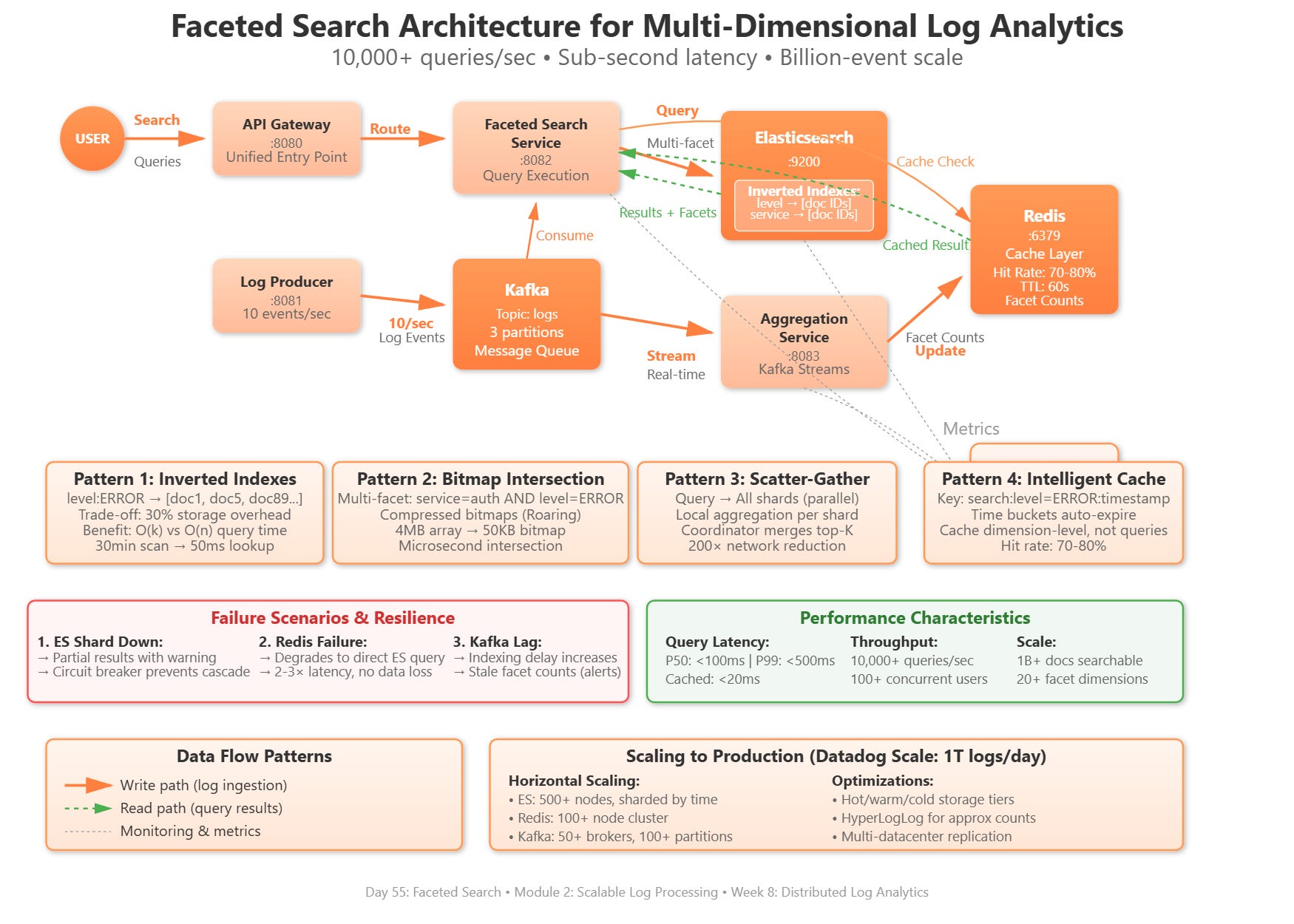
Today we implement a production-grade faceted search system that enables simultaneous filtering across multiple dimensions of log data:
Distributed faceted index with Elasticsearch supporting 10,000+ queries/sec
Real-time facet aggregation computing filter counts across billions of log entries
Multi-dimensional filtering enabling complex queries like “ERROR logs from service=auth AND host=prod-* in last 15 minutes”
Intelligent caching layer with Redis reducing repeated aggregation overhead by 80%
Why This Matters: The Search at Scale Challenge
When Datadog ingests 1 trillion log events daily, users don’t just search for text—they filter by 20+ dimensions simultaneously: service name, environment, log level, HTTP status code, error type, region, host, container ID, and custom tags. Each facet must show real-time counts: “42,385 ERROR logs, 8,234 from auth-service, 3,102 in us-east-1.”
The naive approach—scanning all logs for each dimension—would require petabytes of I/O per second. Instead, production systems use inverted indexes, bitmap intersection, and distributed aggregation to deliver sub-second faceted search across massive datasets. Splunk’s faceted search handles 100,000+ concurrent users filtering terabytes of logs, while Elastic’s distributed aggregation framework powers real-time analytics for half of Fortune 500 companies.
The architectural challenge: how do you maintain accurate facet counts while ingesting 500,000 events/second, support complex boolean queries with 10+ filters, and cache strategically when facet distributions change every second? Today’s lesson implements the patterns that make billion-event search systems feel instantaneous.
System Design Deep Dive
1. Inverted Indexes: The Foundation of Faceted Search
Traditional log storage organizes by time: 2024-01-28 10:00:00 | ERROR | auth-service | Login failed. Faceted search requires the inverse: given level=ERROR, which logs match? Elasticsearch and Solr build inverted indexes mapping each facet value to document IDs:
service:auth-service → [doc1, doc5, doc89, doc234, ...]
level:ERROR → [doc1, doc12, doc89, doc156, ...]
region:us-east-1 → [doc5, doc12, doc234, ...]
Trade-off Analysis: Inverted indexes consume 30-40% additional storage but reduce faceted query time from O(n) full scans to O(k) where k is the result set size. For 1 billion logs, this transforms a 10-minute scan into a 50ms index lookup. The cost: write amplification. Each log ingestion updates multiple indexes—one per facet. At scale, Datadog uses LSM-tree indexes (like Lucene) that batch writes and compact asynchronously, trading slightly stale facets (1-2 second lag) for 10x better write throughput.
2. Bitmap Intersection: Combining Multiple Facets
When users query service=auth AND level=ERROR AND region=us-east-1, the system must intersect three result sets. The naive approach iterates through each set sequentially—O(n1 + n2 + n3). Production systems use compressed bitmaps (Roaring Bitmaps) for bitwise AND operations completing in microseconds.
For 1 million matching document IDs, a sorted integer array consumes 4MB. A compressed bitmap uses 50KB with O(1) intersection. Twitter’s search infrastructure reduced facet query latency by 90% switching from hash-set intersection to roaring bitmaps. The pattern: represent document IDs as bit positions in a bitmap, use hardware-accelerated SIMD instructions for parallel intersection.
Failure Mode: Sparse bitmaps (few set bits in large ranges) compress poorly and waste memory. Pinterest’s search team dynamically chooses between bitmaps and skip lists based on result set density—bitmaps for >1% density, skip lists otherwise.
3. Distributed Aggregation: Computing Facet Counts
The hardest part of faceted search isn’t finding matching documents—it’s computing counts for each facet value in real-time. “Show me all ERROR logs AND tell me how many are from each service” requires scanning matching docs and aggregating dimensions.
Elasticsearch’s distributed aggregation uses a scatter-gather pattern:
Scatter: Send query to all shards (partitioned by time or hash)
Local Aggregation: Each shard computes top-K facet values with counts
Gather: Coordinator merges results, re-ranks, and returns final counts
For a query matching 10 million logs across 50 shards, each shard processes 200K docs locally, returns top 1000 facet values. The coordinator merges 50 × 1000 = 50K facet values into final top 1000. This reduces network transfer from 10 million to 50K results—a 200× reduction.
Scalability Bottleneck: Aggregation memory scales with cardinality (distinct facet values), not document count. A field with 1 million unique values requires 1M × 8 bytes = 8MB per shard just for facet counts. LinkedIn’s search infrastructure uses HyperLogLog for approximate counts when exact values aren’t critical—1.5% error with 99% less memory.
4. Intelligent Caching: Reducing Repeated Aggregation
Facet distributions change slowly—the count of ERROR logs fluctuates, but relative proportions (auth-service: 30%, api-service: 25%) remain stable over minutes. Uber’s log search system caches facet aggregations in Redis with 60-second TTLs:
cache_key = "facets:service:level=ERROR:last_15min:20240128T1000"
cache_value = {
  "auth-service": 8234,
  "api-service": 6012,
  "payment-service": 4829
}
The cache hit rate reaches 80% for dashboard queries where users repeatedly filter similar time ranges. Cache invalidation uses time-bucketed keys—cache expires naturally when time window shifts.
Anti-Pattern: Caching final search results per user query. With 20 facets and 10+ values each, the query space explodes to billions of combinations. Cache aggregations at the dimension level (counts per facet), not query level.
5. Query Optimization: Choosing Execution Paths
Not all faceted queries are equal. level=ERROR AND service=auth (matching 0.1% of logs) should execute differently than level!=ERROR AND service!=auth (matching 99.9%). Production query planners use statistics to choose optimal execution:
Strategy 1 - Filter First: For selective filters (matches <5% of docs), retrieve matching doc IDs, then aggregate facets. Used when result set is small.
Strategy 2 - Aggregate First: For broad filters (matches >50%), compute all facet distributions, then filter. Avoids repeated aggregation for exploratory queries.
Elasticsearch’s query planner estimates cardinality using index statistics and chooses execution strategy automatically. Netflix’s search infrastructure reduced P99 latency from 8 seconds to 400ms by implementing cardinality-aware query planning—pre-computing aggregations for high-cardinality fields, streaming results for low-cardinality fields.
Implementation Walkthrough
GitHub Link :
https://github.com/sysdr/sdc-java/tree/main/day55/day55-faceted-search-systemOur system implements faceted search with four services:
1. Faceted Search Service (Spring Boot + Elasticsearch)
The search service maintains Elasticsearch indexes with faceted fields. Each log document includes dimensions as analyzed fields:
@Document(indexName = "logs")
public class LogDocument {
    private String id;
    private Instant timestamp;
    private String level;      // Facet: ERROR, WARN, INFO
    private String service;    // Facet: auth-service, api-service
    private String environment; // Facet: prod, staging
    private String host;       // Facet: prod-01, prod-02
    private String message;    // Full-text searchable
}
The search API accepts multi-dimensional filters and returns both matching logs and facet counts:
@PostMapping("/search")
public FacetedSearchResponse search(@RequestBody SearchRequest request) {
    // Build Elasticsearch query with multiple filters
    BoolQueryBuilder query = QueryBuilders.boolQuery();
    request.getFilters().forEach((field, value) ->
        query.filter(QueryBuilders.termQuery(field, value))
    );

    // Add facet aggregations for each dimension
    SearchSourceBuilder searchBuilder = new SearchSourceBuilder()
        .query(query)
        .size(request.getLimit())
        .aggregation(AggregationBuilders.terms("by_level").field("level"))
        .aggregation(AggregationBuilders.terms("by_service").field("service"))
        .aggregation(AggregationBuilders.terms("by_environment").field("environment"));

    // Execute distributed query across all shards
    SearchResponse response = elasticsearchClient.search(searchBuilder);

    return buildFacetedResponse(response);
}
2. Aggregation Service (Kafka Streams)
Real-time facet counts flow through a Kafka Streams aggregation pipeline. As logs ingress, the service maintains materialized views of facet distributions:
@Bean
public KStream<String, LogEvent> buildFacetAggregations(StreamsBuilder builder) {
    return builder.stream("logs")
        .groupBy((key, log) -> log.getService())
        .windowedBy(TimeWindows.of(Duration.ofMinutes(5)))
        .count(Materialized.as("service-counts"))
        .toStream()
        .to("facet-aggregations");
}
These pre-computed aggregations seed the cache, reducing query-time aggregation overhead.
3. Cache Layer (Redis)
Facet aggregations cache in Redis with composite keys capturing query dimensions:
public Map<String, Long> getCachedFacets(String field, Map<String, String> filters) {
    String cacheKey = buildFacetCacheKey(field, filters);
    Map<Object, Object> cached = redisTemplate.opsForHash().entries(cacheKey);

    if (!cached.isEmpty()) {
        return cached.entrySet().stream()
            .collect(Collectors.toMap(
                e -> e.getKey().toString(),
                e -> Long.parseLong(e.getValue().toString())
            ));
    }

    // Cache miss - compute from Elasticsearch
    Map<String, Long> facets = computeFacetsFromElasticsearch(field, filters);
    redisTemplate.opsForHash().putAll(cacheKey, facets);
    redisTemplate.expire(cacheKey, Duration.ofMinutes(1));
    return facets;
}
4. Query Planning
Before executing, the system estimates result set size using Elasticsearch count API and chooses execution strategy:
public SearchStrategy chooseStrategy(SearchRequest request) {
    long estimatedMatches = elasticsearchClient.count(buildQuery(request));
    long totalDocs = elasticsearchClient.count(matchAllQuery());
    double selectivity = (double) estimatedMatches / totalDocs;

    // <5% of docs: filter-first strategy (retrieve docs, then aggregate)
    if (selectivity < 0.05) {
        return SearchStrategy.FILTER_FIRST;
    }
    // >50% of docs: aggregate-first strategy (compute facets, then filter)
    else if (selectivity > 0.50) {
        return SearchStrategy.AGGREGATE_FIRST;
    }
    // Medium selectivity: standard scatter-gather
    return SearchStrategy.SCATTER_GATHER;
}
Working Demo Link:
Production Considerations
Performance Optimization: Elasticsearch heap size must accommodate aggregation memory. For 100M unique facet values per shard, allocate 4GB heap minimum. Monitor indices.fielddata.memory_size and implement circuit breakers to prevent OOM during high-cardinality aggregations.
Facet Explosion: Users creating custom tags can introduce unbounded cardinality. Implement dynamic field limits—Splunk restricts to 10,000 unique values per facet per day. Beyond that, treat as full-text searchable but not faceted.
Failure Scenarios: When Elasticsearch shards become unavailable, return partial results with a “incomplete data” warning rather than failing completely. Netflix’s search UI shows “Search results from 45/50 datacenters” during partial outages, maintaining user trust through transparency.
Monitoring: Track facet cache hit rates (target >70%), P99 aggregation latency (target <500ms), and Elasticsearch heap usage (alert above 85%). Set up alerts for abnormal cardinality growth indicating potential facet explosion attacks or bugs.
Scale Connection: FAANG-Level Faceted Search
Datadog processes 100,000 faceted search queries per second across 1 trillion daily log events. Their distributed search cluster uses 500+ Elasticsearch nodes, each maintaining sharded time-series indexes. Facet aggregations execute in parallel across shards with results merged in <200ms. They cache aggregations in a distributed Redis cluster with 100+ nodes, achieving 85% cache hit rates for common queries.
Elastic Cloud powers faceted search for companies like Tinder, Slack, and Walmart. Their most demanding workload—Walmart’s inventory search—handles 50,000 queries/sec with 15+ simultaneous facets across 500 billion documents. The system uses Elasticsearch’s frozen tier to archive old indexes while maintaining query support, reducing storage costs by 90%.
Next Steps
Tomorrow we implement real-time indexing with minimal latency, building sub-second indexing pipelines that make logs searchable within 100ms of generation—the final piece for production-grade observability.