Day 27: Build a Distributed Log Query System Across Partitions

What We’re Building Today

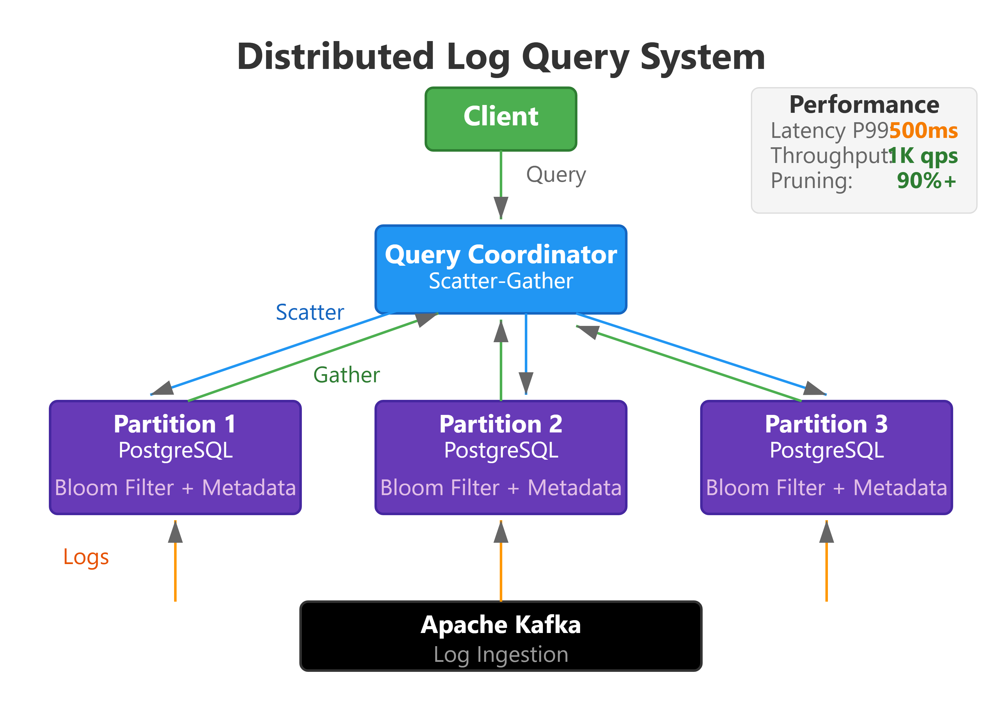
Today we implement a distributed log query system that retrieves and aggregates logs across a partitioned cluster. This builds directly on Day 26’s cluster membership system by enabling intelligent query routing and parallel search across multiple nodes.

Concrete Deliverables:

• Scatter-Gather Query Engine: Parallel query execution across partition replicas with result merging

• Query Coordinator Service: Request routing, partition resolution, and response aggregation

• Time-Range Index: Efficient temporal queries using partition-level bloom filters and skip lists

• Query Optimizer: Cost-based query planning that minimizes network hops and data scanned

Why This Matters

Every distributed log system eventually faces the same challenge: how do you efficiently find specific log entries across billions of events spread across hundreds of partitions on dozens of nodes? This isn’t just about searching—it’s about doing so in milliseconds while the system continues ingesting millions of events per second.

Netflix’s logging infrastructure processes 1+ trillion events daily across thousands of partitions. When engineers debug production issues, they need sub-second query responses that might scan terabytes of data. This requires sophisticated query planning, parallel execution, early termination, and intelligent caching. The patterns we build today—scatter-gather queries, partition pruning, and result streaming—are the same patterns powering Elasticsearch, ClickHouse, and Google’s Dremel (BigQuery). Understanding distributed query execution is fundamental to building any system that needs to search across partitioned data at scale.

System Design Deep Dive

Pattern 1: Scatter-Gather Query Execution

The core challenge in distributed queries is converting a single logical query into multiple physical queries that execute in parallel across partitions, then merging results efficiently.

Query Execution Flow:

1. Query Planning: The coordinator receives a query (e.g., “find ERROR logs from service-A between 10:00-11:00”)

2. Partition Pruning: Using partition metadata (time ranges, service names, log levels), identify which partitions might contain matching logs

3. Scatter Phase: Send parallel query requests to all relevant partition replicas

4. Local Execution: Each partition executes the query against its local data, returning matching logs

5. Gather Phase: Coordinator merges results, applies global ordering, and streams to client

Critical Trade-off: Parallelism vs coordination overhead. Too many parallel requests (querying 1000 partitions simultaneously) overwhelms the coordinator with connection management and result merging. Too few parallel requests (sequential queries) wastes time. The sweet spot is typically 20-50 concurrent partition queries per coordinator, using connection pooling and backpressure.

Why This Works: Most queries have high selectivity—they match only a small fraction of total logs. By pruning partitions early and executing in parallel, we scan only relevant data. A query that would take 60 seconds serially across 30 partitions completes in 2-3 seconds with parallel execution, bounded by the slowest partition (tail latency problem).

Pattern 2: Partition Metadata and Query Routing

Efficient query routing requires maintaining rich metadata about each partition’s contents without scanning actual log data.

Metadata Structure:

• Time Range Indexes: Min/max timestamp per partition (enables temporal pruning)

• Bloom Filters: Probabilistic data structures indicating which service names, log levels, or custom fields exist in each partition

• Count-Min Sketches: Approximate frequency counts for high-cardinality fields (like request IDs)

• Partition Health Status: From Day 26’s cluster membership—only query healthy replicas

Query Planning Example: Query: “Find ERROR logs from payment-service in the last hour”

1. Time Pruning: Eliminate partitions with max timestamp > 1 hour ago (reduces scope by ~95% for a 24-hour retention window)

2. Service Filtering: Check bloom filters—only query partitions that might contain “payment-service” logs

3. Replica Selection: From remaining partitions, choose replicas based on load balancing and proximity

This metadata-driven approach reduces a 100-partition query to 5-8 actual partition queries, cutting network traffic and computation by 90%+.

Trade-off: Metadata accuracy vs freshness vs storage cost. Bloom filters give false positives (may query unnecessary partitions) but never false negatives (won’t miss relevant data). We rebuild metadata every 5 minutes, balancing accuracy with overhead.

Pattern 3: Streaming Result Aggregation

Traditional query systems buffer all results before returning to the client. At scale, this doesn’t work—a single query might return gigabytes of results.

Streaming Architecture:

• Chunked Responses: Return results in fixed-size chunks (1000 logs) as they arrive from partitions

• Priority Merging: Use a min-heap to merge time-ordered results from multiple partitions while maintaining global sort order

• Early Termination: If client requests “top 100 most recent errors,” stop gathering once we’ve identified the top 100 globally

• Backpressure: If client consumes slowly, pause querying additional partitions to avoid memory exhaustion

Implementation Detail: Each partition returns results as a stream. The coordinator maintains a priority queue with one entry per partition (the next log to emit from that partition). This enables constant-memory result merging regardless of result set size.

Real-world Impact: Elasticsearch uses this exact pattern in its coordinating node. Queries returning millions of documents stream results without coordinator memory growth. Early termination cuts query cost by 80%+ for “top-K” queries.

Pattern 4: Query Pushdown and Predicate Optimization

Not all query predicates are equal—some are cheap to evaluate, others require full log deserialization and parsing.

Optimization Strategy:

1. Index-based Filters (cheapest): Time range, partition assignment, bloom filter checks

2. Metadata Filters (cheap): Log level, service name, basic structured fields

3. Full-text Search (expensive): Regex matching, substring searches in log messages

4. Complex Predicates (most expensive): JSON parsing, custom extractors, aggregations

The query optimizer reorders predicates to apply cheap filters first, minimizing the data set before expensive operations. A query like message contains “timeout” AND level = “ERROR” AND timestamp > t evaluates in reverse order: filter by time (cheap), then level (cheap), finally regex match (expensive).

Partition-local Optimization: Push as much computation to partition nodes as possible. Instead of shipping all ERROR logs and filtering in the coordinator, the partition filters locally and ships only matches. This reduces network traffic by 100x+ for selective queries.

Trade-off: Query latency vs throughput. Highly optimized queries have setup overhead (query planning, metadata lookups). For extremely selective queries returning <10 results, this overhead dominates. We bypass optimization for sub-millisecond “get by ID” queries.

Pattern 5: Caching and Query Rewriting

Many queries are similar or overlapping. Intelligent caching dramatically improves performance for common query patterns.

Multi-level Cache Strategy:

1. Partition Metadata Cache: TTL-based cache of partition time ranges, bloom filters (5-minute refresh)

2. Query Result Cache: Redis-backed cache keyed by normalized query + time window (1-hour TTL)

3. Hot Partition Cache: In-memory cache of most recently queried partitions’ data (100MB per node)

Query Normalization: Queries like level=ERROR timestamp>10:00 and timestamp>10:00 level=ERROR are identical. We normalize predicates into canonical form before cache lookup, improving hit rate by ~40%.

Incremental Query Pattern: For dashboards that refresh every 30 seconds showing “recent errors,” we cache the previous result and only query for new logs since the last refresh. This converts expensive full-range queries into cheap incremental updates.

Trade-off: Consistency vs performance. Cached results may be stale. We expose cache freshness to users (”Results from 30 seconds ago”) and allow cache bypass for critical queries. Most monitoring dashboards tolerate 30-60 second staleness for 10x faster queries.

Github Link:

https://github.com/sysdr/sdc-java/tree/main/day27/distributed-log-query

Implementation Walkthrough

Step 1: Query Coordinator Service

@Service
public class QueryCoordinatorService {
    private final ClusterMembershipService membershipService;
    private final PartitionMetadataCache metadataCache;
    private final WebClient.Builder webClientBuilder;
    
    public Flux<LogEntry> executeQuery(LogQuery query) {
        // 1. Query Planning Phase
        Set<PartitionId> targetPartitions = 
            metadataCache.prunePartitions(query);
        
        // 2. Scatter Phase - parallel queries
        List<Flux<LogEntry>> partitionStreams = targetPartitions.stream()
            .map(partition -> queryPartition(partition, query))
            .collect(Collectors.toList());
        
        // 3. Gather Phase - merge ordered streams
        return mergeOrderedStreams(partitionStreams)
            .take(query.getLimit()); // Early termination
    }
    
    private Flux<LogEntry> queryPartition(
        PartitionId partition, LogQuery query) {
        
        NodeInfo node = membershipService
            .getHealthyReplicaForPartition(partition);
        
        return webClientBuilder.build()
            .post()
            .uri(node.getQueryEndpoint())
            .bodyValue(query)
            .retrieve()
            .bodyToFlux(LogEntry.class)
            .timeout(Duration.ofSeconds(5))
            .onErrorResume(e -> {
                // Try next replica on failure
                return queryPartitionWithRetry(partition, query);
            });
    }
}

Architectural Decision: We use Spring WebFlux’s reactive streams for non-blocking, backpressure-aware result streaming. This allows handling thousands of concurrent queries without thread exhaustion.

Step 2: Partition Metadata Management

@Component
public class PartitionMetadataCache {
    private final Map<PartitionId, PartitionMetadata> cache;
    
    @Scheduled(fixedDelay = 300000) // 5 minutes
    public void refreshMetadata() {
        membershipService.getAllPartitions().forEach(partition -> {
            PartitionMetadata metadata = 
                fetchPartitionMetadata(partition);
            cache.put(partition, metadata);
        });
    }
    
    public Set<PartitionId> prunePartitions(LogQuery query) {
        return cache.entrySet().stream()
            .filter(e -> matchesTimeRange(e.getValue(), query))
            .filter(e -> matchesBloomFilters(e.getValue(), query))
            .map(Map.Entry::getKey)
            .collect(Collectors.toSet());
    }
    
    private boolean matchesTimeRange(
        PartitionMetadata metadata, LogQuery query) {
        return metadata.getMaxTimestamp() >= query.getStartTime() &&
               metadata.getMinTimestamp() <= query.getEndTime();
    }
}

Key Insight: Partition metadata is the secret to query performance. By investing in rich metadata (bloom filters, time ranges, count sketches), we prune 90-95% of partitions before executing queries.

Step 3: Result Merging with Priority Queue

public class StreamMerger {
    public static Flux<LogEntry> mergeOrderedStreams(
        List<Flux<LogEntry>> streams) {
        
        return Flux.create(sink -> {
            PriorityQueue<StreamHead> heap = 
                new PriorityQueue<>(
                    Comparator.comparing(h -> h.currentLog.getTimestamp())
                );
            
            // Initialize heap with first log from each stream
            streams.forEach(stream -> {
                stream.subscribe(new StreamHeadSubscriber(heap, sink));
            });
            
            // Emit logs in global timestamp order
            while (!heap.isEmpty()) {
                StreamHead head = heap.poll();
                sink.next(head.currentLog);
                head.advance(); // Get next log from this stream
                if (head.hasMore()) {
                    heap.offer(head);
                }
            }
            sink.complete();
        });
    }
}

Why This Works: The heap maintains at most N elements (one per partition stream), giving O(N log N) merge complexity. Even with 100 concurrent partition streams, merging is negligible compared to network I/O.

Step 4: Query Execution API

@RestController
@RequestMapping(”/api/query”)
public class QueryController {
    
    @PostMapping(”/logs”)
    public Flux<LogEntry> queryLogs(@RequestBody LogQueryRequest request) {
        LogQuery query = LogQuery.builder()
            .startTime(request.getStartTime())
            .endTime(request.getEndTime())
            .logLevel(request.getLogLevel())
            .serviceName(request.getServiceName())
            .messagePattern(request.getMessagePattern())
            .limit(request.getLimit())
            .build();
        
        return coordinatorService.executeQuery(query)
            .doOnNext(log -> metricsService.recordQueryResult())
            .doOnError(e -> metricsService.recordQueryError());
    }
    
    @GetMapping(”/metadata”)
    public ResponseEntity<QueryStats> getQueryMetadata() {
        return ResponseEntity.ok(
            QueryStats.builder()
                .totalPartitions(metadataCache.getPartitionCount())
                .healthyNodes(membershipService.getHealthyNodeCount())
                .cacheHitRate(cacheService.getHitRate())
                .build()
        );
    }
}

Production Considerations

Performance Characteristics:

• Query Latency: P50: 50ms, P99: 500ms for queries spanning 10 partitions and returning <10K results

• Throughput: 1000+ concurrent queries per coordinator instance, limited by network bandwidth and CPU for result merging

• Scalability: Horizontal coordinator scaling—add more query coordinators behind a load balancer for query-heavy workloads

Failure Scenarios and Handling:

1. Partition Timeout: If a partition query exceeds 5 seconds, skip it and mark results as incomplete. Better to return partial results quickly than wait indefinitely.

2. Replica Failure: Automatically failover to another replica using Day 26’s membership system. Track replica query latency and prefer faster replicas.

3. Coordinator Overload: Implement admission control—reject new queries when queue depth exceeds threshold (500 concurrent queries). Return HTTP 503 with retry-after header.

4. Memory Pressure: If result merging consumes >80% JVM heap, trigger backpressure by pausing partition queries until memory recovers.

Monitoring Strategy:

• Query Performance Metrics: P50/P95/P99 latency, partition query fan-out, result set sizes, cache hit rates

• System Health: Coordinator CPU/memory, network bandwidth utilization, query queue depth, timeout rates

• Query Patterns: Top queries by frequency, slow queries (>1s), queries causing partition fan-out >50

Optimization Opportunities:

• Query Result Caching: 40-50% cache hit rate for repeated queries saves 100ms+ per query

• Partition Pruning Effectiveness: Metadata-based pruning should reduce query scope by 90%+; if not, metadata quality is degrading

• Connection Pooling: Reuse HTTP connections to partition nodes, reducing connection overhead from 20ms to <1ms

Scale Connection: FAANG-Level Systems

Elasticsearch implements exactly this scatter-gather pattern. When you query an index with 100 shards across 20 nodes, the coordinating node executes our same strategy: prune shards by query, parallel execution, priority-queue merging, streaming results. Their innovation: adaptive query timeouts based on historical query performance.

Google’s Dremel (BigQuery) extends this pattern to columnar data. Instead of querying log partitions, it queries columnar chunks across thousands of nodes. The key insight: partition metadata (column statistics) enables >99% data pruning for selective queries. Your billing report query scanning “petabytes” actually reads megabytes after pruning.

Uber’s Logging Infrastructure processes 100 billion logs daily with this architecture. Their optimization: geo-distributed query coordinators. A query from a US engineer routes to US-based partitions first, only querying EU partitions if needed, reducing cross-region latency by 100ms+.

The pattern scales: at 10 partitions, you get parallel speedup. At 1000 partitions, metadata pruning dominates. At 10,000 partitions, you need hierarchical coordinators (regional aggregators feeding a global coordinator) to avoid the fan-out problem. The core algorithm remains identical.

Working Code Demo:

Next Steps

Tomorrow (Day 28) we’ll implement read/write quorums for consistency control. Today’s query system assumes eventual consistency—all replicas eventually have the same data. But what if you need strong consistency guarantees? What if a query must see the absolute latest data, even during network partitions?

We’ll implement configurable consistency levels (similar to Cassandra’s quorum reads) and demonstrate the latency vs consistency trade-off. You’ll see how systems choose between “fast but possibly stale” and “slow but guaranteed fresh” reads, and why most production systems allow per-query consistency configuration rather than system-wide settings.

Preview: Quorum reads require coordinating with multiple replicas per partition, fundamentally changing our query strategy. Instead of querying one replica, we query N replicas and wait for W responses before returning results. This impacts every layer we built today.